Timsort Sorting Algorithm

What is Timsort Algorithm?

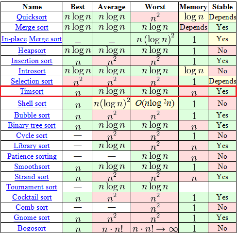
Unlike “bubble” or “insertion” sorting, Timsort is rather new — it was invented in 2002 by Tim Peters (and named after him). It has been a standard sorting algorithm in Python, OpenJDK 7 and Android JDK 1.5 ever since. And to understand why, one should only look at this Wikipedia table.

In a seemingly huge choice of algorithms, the table offers only seven proper ones (with theO(n logn) complexity as the average or the worst case ), out of which only two can boast stability and O(n) complexity as the best case. One of the two is the good old Tree sort, and the second is Timsort.

The algorithm is based on the idea that in the real world the sorted data array contain ordered (no matter how: non-descending or descending) sub-arrays. And often it really is so. With such data Timsort goes ahead of all other algorithms in software engineering.

Straight to the Matter

Please, do not expect any complex mathematical discoveries. The thing is that in reality Timsort is not a standalone algorithm but a hybrid, an efficient combination of a number of other algorithms, seasoned with the author’s ideas. The mechanism of the algorithm can be briefly explained as follows:

• A particular algorithm is used to split the input array into sub-arrays.
• Each sub-array is sorted with a simple Insertion Sort.
• The sorted sub-arrays are merged into one array with the use of Merge Sort. As usual, the devil hides in the details, namely, in the algorithm in p. 1 and the merge sort modification in p. 3.

The Algorithm

Definitions

• N: the length of the input array
• run: an ordered sub-array in the input array. At the same time, the order is non-descending or strictly descending, i.e. “a0 ≤ a1 ≤ a2 ≤ …» or «a0 > a1 > a2 > …”
• minrun: as it was said above, in the first step of the algorithm, the input array is split into runs. minrun is a minimum length of such run. This number is calculated by a certain logics from the N number.

Step 0. Calculation of the Minrun.

The minrun number is determined based on the N, by the following principles:

• It shouldn’t be too long as the minrun will later be subjected to insertion sort, which is effective for short runs.
• It shouldn’t be too short, as, the shorter the run, the more runs will have to be merged in the next step.
• It would be good if N \ minrun was a power of 2 (or close to it). This requirement results from the fact that the merge sort performs best on the runs of about the same length.

Here, the author refers to his own experiments, showing that with minrun > 256, principle 1 is not satisfied, and with minrun < 8, principle 2 is not satisfied, and the most performing lengths range from 32 to 65. Exception: if N < 64, then minrun = N and Timsort turns into a simple merge sort. At this point, the minrun calculation algorithm is as simple as a piece of cake: take the six most significant bits out of N and add one, if the remaining least significant bits contain at least one off bit. An approximate code will look somewhat like this:

    int GetMinrun(int n)
    {
        int r = 0;  /* becomes 1 if the least significant bits contain at least one off bit */
        while (n >= 64) {
            r |= n & 1;
            n >>= 1;
        }
        return n + r;
    }

Step 1. Splitting into Runs and Their Sorting.

So, at this stage, there is an input array with N size and a calculated minrun. The algorithm for this step:

• The base address of the current element is set at the beginning of the input array.
• Starting with the current array, search for the run (an ordered array) in the input array. By definition, this run will definitely include the current element and the one that follows, but further on it’s pure luck. If the final array is descending, the elements are ordered in a non-descending order (it’s a simple serial algorithm, it’s just that we move from both sides to the centre, changing the places of the elements).
• If the current run is smaller than the minrun, take the number of elements that follow the found run equal to the minrun — size(run). Thus, the final run will be the size of the minrun or more, a part of which (ideally all of it) is ordered.
• Then this run is insertion sorted. As this run is small and partially ordered, the sorting is fast and highly performing.
• The base address of the current element is set at the element following this run.
• If the end of the input array has not been reached, go to point 2, otherwise it is the end of this step.

Step 2. Merge

At this stage, there is an input array split into runs. If the data in the input array were close to random, the run size is close to minrun, and if the data had ordered ranges (the algorithm application requirement lets us hope for it), the run size exceeds minrun. Now, these runs need to be combined to receive the final and completely ordered array, and in the course of it, two requirements have to be satisfied:

• There should be combined runs of relatively equal size (this way it will be more efficient).
• The algorithm stability should be maintained, i.e. no useless shifts (e.g. two consecutive equal numbers should not exchange places).

This is achieved in the following way:

• Create an empty pair stack <run base address>–<run size>. Take the first run.
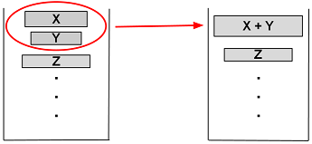
• Add a few data to the stack <base address>–<size> to the current run.
• Assess whether the current run should be merged with the preceding one. To do this, check where the two requirements are satisfied (say, X, Y and Z are three top runs in the stack): X > Y + Z Y > Z
• If one of the requirements is not satisfied, array Y is merged with the smallest of arrays X and Z. This step is performed until both requirements are satisfied or until all data is ordered.
• For any unconsidered runs, take the next and go point 2. Otherwise, it is the end.

The aim of this procedure is to keep the balance, i.e. the changes will look as follows:

thus, run sizes fit for further merge sorting. Imagine an ideal case: there is a run with the size of 128, 64, 32, 16, 8, 4, 2 and 2 (let’s forget for a while about the requirement that run size ≥minrun). In this case there won’t be any merges until the last two runs do not meet, and after that seven perfectly balanced merges will be performed.

Runs Merging

As you remember, in step two of the algorithm, we were merging two runs into an ordered one. The two consecutive runs are always merged. To merge them an additional memory is used.

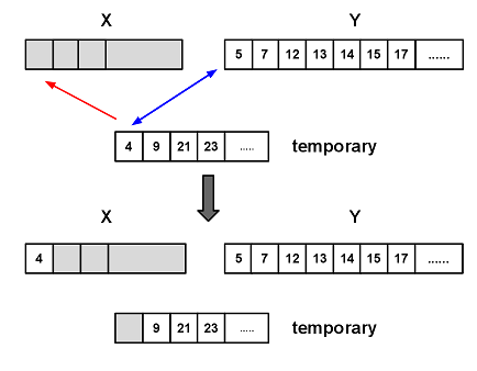
• A temporary run is created with a size of the smallest of the merged runs.
• Copy the shortest run into the temporary one.
• Mark the current position with the first elements of the large and temporary arrays.
• In each following step compare the elements in the large and temporary arrays and move the smaller into a new sorted array. Move the base address of the element in the array, where the element was taken from.
• Repeat step 4 until one of the arrays runs out.
• Add all elements of the remaining run to the end of the new one.

Modifications to the Merging Sort

All seems perfect in the above merge sort. Except for one thing: imagine the merge of such two arrays:

A = {1, 2, 3,…, 9999, 10000}

B = { 20000, 20001, …., 29999, 30000}

The above procedure will work for them too, but at each step four, one comparison and one moving should be performed to give 10000 comparisons and 10000 moves. Timsort offers here a modification called galloping. It means the following:

• Start the merge sort as described above.
• At each moving of an element from the temporary or large run to the final one, the run where the element was moved from is recorded.
• If a number of elements (in this representation of the algorithm this number equals 7) was moved from one and the same run, it can be assumed that the next element will also come from the same run. To prove it, the galloping mode is switched, i.e. go through the run that is expected to supply the next set of data with a binary search (remember that the array is ordered and we have all rights for binary search) to find the current element from the other merged run. The binary search is more efficient than the linear one, thus the number of searches will be much smaller.
• Finally, when the data in the supplying run do not fit (or having reached the run end), this data can be moved in a bulk (which can be more efficient than moving separate elements).

The explanation can be a bit vague, so let’s have a look at the example: A = {1, 2, 3,…, 9999, 10000} B = { 20000, 20001, …., 29999, 30000}

• In the first seven iterations, numbers 1, 2, 3, 4, 5, 6 and 7 from run A are compared with number 20000 and, after 20000 is found to be greater, they are moved from array A to the final one.
• Starting with the next iteration, the galloping mode is switched on: number 20000 is compared in sequence with numbers 8, 10, 14, 22, 38, n+2^i, …, 10000 from run A. As you can see, the number of such comparisons will be far less than 10000.
• When run A is empty, it is known that it is smaller than run B (we could also have stopped somewhere in the middle). The data from run A is moved to the final one, and the procedure is repeated.

That’s the end of the algorithm.

READ ALSO:

• BlueStacks + Eclipse: Speeding up Debugging and Testing of Android Applications
• Interception of HTTPS Traffic between Android Device and External Server
• Code Review and the Theory of Probability